Understanding 10x Xenium Data Analysis
Overview of Spatial Transcriptomics (ST)
Traditional single-cell RNA sequencing (scRNA-seq) dissociates cells and profiles gene expression at single cell resolution. It is able to capture the heterogeneity within tissues and gives high resolution insight into cellular functions.
While this type of data can be used to analyze variations in gene expression, it lacks the spatial information for cells, which adds a dimension of information. Enter ‘Spatial Transcriptomics’ (ST)! After being named the Method of the year 2020[1] ST has revolutionized our ability to understand biology by capturing the spatial information. Having spatial context allows us to look deeper into cell-cell interactions, cellular niches, and various microenvironments across conditions.
Over the last few years, spatial transcriptomics technologies have advanced rapidly and each come with various advantages. Detailed table can be found here.
Overview of Xenium
Xenium is a single-cell resolution technology commercialized by 10x genomics in 2023. It uses RNA based transcripts and can target up to 5000 genes. It captures transcripts at subcellular level. 10x also has nuclear and cell membrane staining which are used for cell segmentation downstream, as compared to the default which only has nuclear staining and cells are detected based on cell-boundary expansion after nucleus segmentation[2].
A few caveots to note for xenium data are that the data generation for large number of samples for entire tissue sections is expensive. So the general practice is to build a Tissue Microarray (TMA) with 30-45 cores of 1.5mm-2mm diameter. Selecting these cores haphazardly can induce data bias as it captures a small section of the condition to be captured. So, building TMA with help of expert pathalogists is a necessary step. Ex: When it comes to studying cancer, the most interesting parts are boundaries between either tumor and immune cells or tumor and stromal cells. These regions are full of potential, allowing us to dive deeper into finding interactions and spatial structures between in such regions.
Understand 10x output files
The Xenium analyzer has numerous outputs we only need some of them to start with data analysis. Here are those files:
| File Type | File and Description |
|---|---|
| Cell summary | cells.parquet: Cell summary file in Parquet format. |
| Cell-feature matrix | cell_feature_matrix.h5: Cell-feature matrix file in HDF5 format. |
Table 2: Xenium Onboard Analysis Output Files[3]
Getting started with data analysis
I will use the Human Lung Cancer with Xenium Multimodal Cell Segmentation data for showcase.
We can get started once Xenium_V1_humanLung_Cancer_FFPE_outs.zip is downloaded.
unzip -d data Xenium_V1_humanLung_Cancer_FFPE_outs.zip
Installing necessary libraries
pip install anndata scanpy squidpy
Loading the data as an AnnData object from raw output files
import os
import pandas as pd
import anndata as ad
import scanpy as sc
import squidpy as sq

import matplotlib.pyplot as plt
plt.rcParams['figure.dpi'] = 250        # increase figure dpi for better quality plots

# load count matrix
adata = sc.read_10x_h5('data/cell_feature_matrix.h5')

# load cells metadata
cells = pd.read_parquet('data/cells.parquet')
cells.index = cells['cell_id']
cells.drop(['cell_id'], inplace=True, axis=1)

adata.obs = cells.copy()

# set spatial info
adata.obsm["spatial"] = adata.obs[["x_centroid", "y_centroid"]].copy().to_numpy()

adata.write_h5ad('objects/xenium_adata.h5ad')
Understanding xenium data structure
AnnData object with n_obs × n_vars = 162254 × 377
    obs: 'x_centroid', 'y_centroid', 'transcript_counts', 'control_probe_counts',
    'control_codeword_counts', 'unassigned_codeword_counts', 'deprecated_codeword_counts',
    'total_counts', 'cell_area', 'nucleus_area'
    var: 'gene_ids', 'feature_types', 'genome'
    obsm: 'spatial'
adata.obs stores the metadata. adata.var stores information about the genes on the panel. More information on AnnData structure can be found here. x_centroid and y_xentroid are the x and y coordinates of the cells.
QC
print(f'Shape of object before filtering: {adata.shape}')

sc.pp.calculate_qc_metrics(adata, percent_top=None, inplace=True)

sc.pp.filter_cells(adata, min_counts=10)

print(f'Shape of object after filtering: {adata.shape}')
As part of quality control we drop cells with n_genes_by_counts < 10.
AnnData object with n_obs × n_vars = 154472 × 377
    obs: 'x_centroid', 'y_centroid', 'transcript_counts', 'control_probe_counts',
    'control_codeword_counts', 'unassigned_codeword_counts',
    'deprecated_codeword_counts', 'total_counts', 'cell_area', 'nucleus_area',
    'n_genes_by_counts', 'log1p_n_genes_by_counts', 'log1p_total_counts', 'n_counts'
    var: 'gene_ids', 'feature_types', 'genome', 'n_cells_by_counts',
    'mean_counts', 'log1p_mean_counts', 'pct_dropout_by_counts', 'total_counts', 'log1p_total_counts'
    obsm: 'spatial'
Shape of object before filtering: (162254, 377)
Shape of object after filtering: (154472, 377)
Referring to this paper we’ll normalize target_sum=100 and log normalize.
# Normalize total
sc.pp.normalize_total(adata, target_sum=100)

# Log-normalize
sc.pp.log1p(adata)
We will apply dimensionality reduction methods
# Run PCA
sc.pp.pca(adata)

# Calculate neighbors
sc.pp.neighbors(adata)

# Leiden clustering
sc.tl.leiden(adata)

# Computing UMAP
sc.tl.umap(adata)
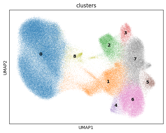
We will plot the UMAP and color on leiden clusters using sc.pl.umap(adata, color='leiden', legend_loc='on data')
NOTE: I have merged some leiden clusters to group similar clusters together in a new column ‘clusters’
Layers of spatial data
Neighborhood enrichment
The reason for spatial data generation is having the x_centroid and y_centroid for each cell. This allows us to build a neighborhood graph.
sq.gr.spatial_neighbors(adata, radius=50, coord_type='generic') # radius in µm
By default this creates an entries ‘spatial_connectivities’ and ‘spatial_distances’ in in adata.obsp.
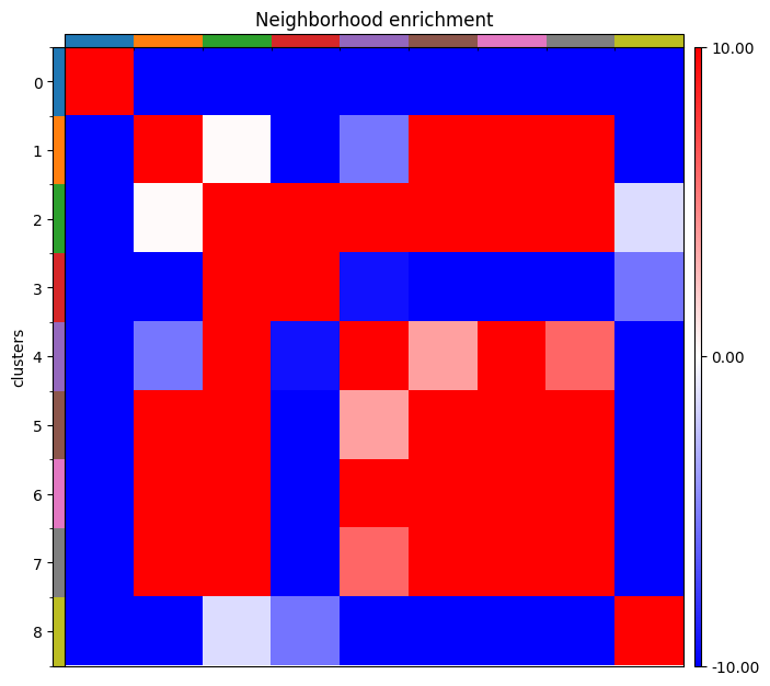
We can now run neighborhood enrichment to see which cells group together using:
# set seed=0 for reproducibility
sq.gr.nhood_enrichment(adata, cluster_key='clusters', seed=0)
Using sq.pl.nhood_enrichment(adata, cluster_key='clusters', cmap='bwr', vmin=-10, vmax=10) we can plot the neighborhood enrichment.
Neighborhood and Proximity scores
Another interesting analysis that is possible with spatial information is looking into neighborhoods at single-cell resolution. Using the method defined in Barkley et al[4].
connections = adata.obsp['spatial_connectivities'].tocsr()

def fetch_neighbors(connections, cell_id):
    row_idx = adata.obs_names.get_loc('cell_name')
    neighbor_idx = connections[row_idx].indices
    return adata.obs_names[neighbor_idx]

def get_neighborhood_score(adata, spot_id, target_column):
    """Returns neighborhood score
    Args:
    adata(anndata.AnnData): input anndata object
    spot_id(str): cell id
    target_column(str): celltype/cluster column
    """
    neighbors = fetch_neighbors(connections, spot_id)
    cluster = adata.obs.loc[neighbors+[spot_id]]
    return cluster[target_column].value_counts() / cluster[target_column].shape[0]

def get_proximity_score(adata, spot_id, target_column):
    """Returns proximity score
    Args:
    adata(anndata.AnnData): input anndata object
    spot_id(str): cell id
    target_column(str): celltype/cluster column
    """
    source = np.array(adata.obs.loc[spot_id, ['x_centroid', 'y_centroid']].values, dtype=np.float64)
    proximity = {}

    centroids = adata.obs.loc[adata.obs.index != spot_id, ['x_centroid', 'y_centroid']].values
    target_celltypes = adata.obs.loc[adata.obs.index != spot_id, target_column]

    for target_oi in np.unique(target_celltypes):
        target_idx = np.where(target_celltypes == target_oi)[0]
        target_coords = np.array(centroids[target_idx], dtype=np.float64)
        distances = np.linalg.norm(target_coords - source, axis=1)
        proximity[target_oi] = 1 / (1 + np.min(distances))
    return pd.Series(proximity)
The paper defines this for visium, the code provided here is updated to support xenium data. We can compare neighborhood and proximity scores between conditions across a cohort or compare these scores between different neighborhoods within the same core.
Lot of work ahead…
QC - filtering cells
Filtering cells using a global threshold for metrics like n_genes_by_counts or total_counts can lead to suboptimal results by discarding biologically relevant cells that appear low-quality in a global context but are consistent with their local tissue environment. This is because global thresholds ignore the inherent spatial structure of tissues, potentially confounding biological variation with technical noise. SpotSweeper[5] addresses this limitation by introducing a spatially aware quality control framework that leverages local neighborhood information to detect outliers based on a zscore.
References
[1] Marx, V. Method of the Year: spatially resolved transcriptomics. Nat Methods 18, 9–14 (2021). https://doi.org/10.1038/s41592-020-01033-y
[2] Xenium In Situ Multimodal Cell Segmentation: Workflow and Data Highlights. https://cdn.10xgenomics.com/image/upload/v1710785020/CG000750_XeniumInSitu_CellSegmentation_TechNote_RevA.pdf
[3] Xenium Output Files at a Glance. https://www.10xgenomics.com/support/software/xenium-onboard-analysis/2.0/tutorials/outputs/xoa-output-at-a-glance
[4] Barkley, D., Moncada, R., Pour, M. et al. Cancer cell states recur across tumor types and form specific interactions with the tumor microenvironment. Nat Genet 54, 1192–1201 (2022). https://doi.org/10.1038/s41588-022-01141-9
[5] Totty, M., Hicks, S.C. & Guo, B. SpotSweeper: spatially aware quality control for spatial transcriptomics. Nat Methods 22, 1520–1530 (2025). https://doi.org/10.1038/s41592-025-02713-3